Combinatorial Test Coverage Measurement

User manual for coverage measurement tool can be found here.
Test coverage is one of the most important topics in software assurance. Users would like some quantitative measure to judge the risk in using a product. For a given test set, what can we say about the combinatorial coverage it provides? With physical products, such as light bulbs or motors, reliability engineers can provide a probability of failure within a particular time frame. This is possible because the failures in physical products are typically the result of physics, such as metal fatigue.

With software the situation is more complex, and many different approaches have been devised for determining software test coverage. With millions of lines of code, or only with a few thousand, the number of paths through a program is so large that it is impossible to test all paths. For each if statement, there are two possible branches, so nif statements in sequence lead to 2ⁿ possible paths, and with loops (while statements) the number of paths is infinite. Thus a variety of measures have been developed to gauge the degree of test coverage. The following are some of the better-known coverage metrics:

• Statement coverage: This is the simplest of coverage criteria – the percentage of statements exercised by the test set. While it may seem at first that 100% statement coverage should provide good confidence in the program, in practice, statement coverage is often considered nearly worthless. At best, less than nearly full statement coverage indicates that a test set is inadequate.


• Decision or branch coverage: The percentage of branches that have been evaluated to both true and false by the test set.


• Condition coverage: The percentage of conditions within decision expressions that have been evaluated to both true and false. Note that 100% condition coverage does not guarantee 100% decision coverage. For example, “if (A || B) {do something} else {do something else}” is tested with [0 1], [1 0], then A and B will both have been evaluated to 0 and 1, but the else branch will not be taken because neither test leaves both A and B false.


• Modified condition decision coverage (MCDC): This is a strong coverage criterion that is required by the US Federal Aviation Administration for Level A (catastrophic failure consequence) software; i.e., software whose failure could lead to complete loss of life. It requires that every condition in a decision in the program has taken on all possible outcomes at least once, and each condition has been shown to independently affect the decision outcome, and that each entry and exit point have been invoked at least once.

Note that the coverage measures above depend on access to program source code. Combinatorial testing, in contrast, is a black box technique. Inputs are specified and expected results determined from some form of specification. The program is then treated as simply a processor that accepts inputs and produces outputs, with no knowledge expected of its inner workings.

Even in the absence of knowledge about a program’s inner structure, we can apply combinatorial methods to produce precise and useful measures. In this case, we measure the state space of inputs. Suppose we have a program that accepts two inputs, x and y, with 10 values each. Then the input state space consists of the 10² = 100 pairs of x and y values, which can be pictured as a checkerboard square of 10 rows by 10 columns. With three inputs, x, y, and z, we would have a cube with 10³ = 1,000 points in its input state space. Extending the example to n inputs we would have a (hard to visualize) hypercube of n dimensions with 10ⁿ points. Exhaustive testing would require inputs of all 10ⁿ combinations, but combinatorial testing could be used to reduce the size of the test set.

Since it is nearly always impossible to test all possible combinations, combinatorial testing is a reasonable alternative. For some value of t, testing all t-way interactions will detect nearly all errors. It is possible that t = n, but recalling the empirical data on failures, we would expect t to be relatively small. Determining the level of level of input or configuration state space coverage can help in understanding the degree of risk that remains after testing. If 90% - 100% of the state space has been covered, then presumably the risk is small, but if coverage is much smaller, then the risk may be substantial. But how should state space coverage be measured? Looking closely at the nature of combinatorial testing leads to several measures that are useful. We begin by introducing what will be called a variable-value configuration.

Definition. For a set of t variables, a variable-value configuration is a set of t valid values for the variables.

Example. Given four binary variables, a, b, c, and d, a=0, c=1, d=0 is a variable-value configuration, and a=1, c=1, d=0 is a different variable-value configuration for the same three variables a, c, and d.

Simple t-way combination coverage

Of the total number of t-way combinations for a given collection of variables, what percentage will be covered by the test set? If the test set is a covering array, then coverage is 100%, by definition, but many test sets not based on covering arrays may still provide significant t-way coverage. If the test set is large, but not designed as a covering array, it is very possible that it provides 2-way coverage or better. For example, random input generation may have been used to produce the tests, and good branch or condition coverage may have been achieved. In addition to the structural coverage figure, it would be helpful to know what percentage of 2-way, 3-way, etc. coverage has been obtained.

Definition. For a given test set for n variables, simple t-way combination coverage is the proportion of t-way combinations of n variables for which all variable-values configurations are fully covered.

Example. Figure 1 shows an example with four binary variables, a, b, c, and d, where each row represents a test. Of the six 2-way combinations, ab, ac, ad, bc, bd, cd, only bd and cd have all four binary values covered, so simple 2-way coverage for the four tests in Figure 1 is 1/3 = 33.3%. There are four 3-way combinations, abc, abd, acd, bcd, each with eight possible configurations: 000, 001, 010, 011, 100, 101, 110, 111. Of the four combinations, none has all eight configurations covered, so 3-way coverage for this test set is 0%.

a	b	c	d
0	0	0	0
0	1	1	0
1	0	0	1
0	1	1	1

Figure 1. An example test array for a system with four binary components

t+k-way combination coverage

A test set that provides some percentage of coverage for t-way combinations will also provide some degree of coverage for t+1-way combinations, t+2-way combinations, etc. This statistic may be useful for comparing two combinatorial test sets. For example, different algorithms may be used to generate 3-way covering arrays. They both achieve 100% 3-way coverage, but if one provides better 4-way and 5-way coverage, then it can be considered a more thorough set.

Definition. For a given test set for n variables, t+k-way combination coverage is the proportion of t+k-way combinations of n variables for which all variable-values configurations are fully covered.

Example. If the test set in Figure 1 is extended as shown in Figure 2, we can extend 3-way coverage. For this test set, bcd is covered, so 2-way coverage is 100%, and 2+1-way = 3-way coverage is 25%.

a	b	c	d
0	0	0	0
0	1	1	0
1	0	0	1
0	1	1	1
0	1	0	1
1	0	1	1
1	0	1	0
0	1	0	0

Figure 2. Eight tests for four binary variables

Configuration coverage

So far we have only considered measures of the proportion of combinations for which all configurations of t variables are fully covered. But when t variables with v values each are considered, each t-tuple has v ^t configurations. For example, in pairwise (2-way) coverage of binary variables, every 2-way combination has four configurations: 00, 01, 10, 11. We can define two measures with respect to configurations:

Definition. For a given set of t variables, configuration coverage is the proportion of variable-value configurations that are covered.

Definition. For a given set of n variables, (p, t)-completeness is the proportion of the C(n, t) combinations that have configuration coverage of at least p.

Example. For Figure 1 above, there are C(4,2) = 6 possible variable combinations and C(4,2) * 2² = 24 possible variable-value configurations. Of these, 19 variable-value configurations are covered and the only ones missing are ab=11, ac=11, ad=10, bc=01, bc=10. But only two, bd and cd, are covered with all 4 value pairs. So for the basic definition of simple t-way coverage, we have only 33% (2/6) coverage, but 79% (19/24) for the configuration coverage metric. For a better understanding of this test set, we can compute the configuration coverage for each of the six variable combinations, as shown in Figure 3. So for this test set, 17% of the variable-value configurations are covered at the 50% level, 50% are covered at the 75% level, and 33% are covered at the 100% level. And, as noted above, for the whole set of tests, 79% of variable-value configurations are covered. All 2-way combinations have at least 50% configuration coverage, so (.50, 2)-completeness for this set of tests is 100%.

Figure 3. The test array covers the six possible 2-way combinations of a, b, c, and d to different levels, as shown in Table 1.

Table 1
Vars	Configurations	Config coverage
ab	00, 01, 10	.75
ac	ac: 00, 01, 10	.75
ad	ad: 00, 01, 11	.75
bc	bc: 00, 11	.50
bd	bd: 00, 01, 10, 11	1.0
cd	cd: 00, 01, 10, 11	1.0

• total 2-way coverage = 19/24  = .79167


• (.50, 2)-completeness = 6/6    = 1.0


• (.75, 2)-completeness = 5/6    = 0.83333


• (1.0, 2)-completeness = 2/6    = 0.33333

Figure 4 is an example of coverage for a 2⁸⁷3²4⁵ set (87 binary, two 3-value, and five 4-value) of input variables (blue=2-way, pink=3-way, yellow=4-way). This particular test set was not a covering array, but pairwise coverage is still quite good, with about 95% of the variables having all possible 2-way configurations covered. Even for 4-way combinations we see that all variables have at least 28% of their configurations covered, and about 25% of them have about 98% or more of 4-way configurations covered.

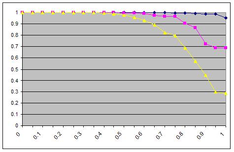
Figure 4. Configuration coverage for 2⁸⁷3²4⁵ inputs.

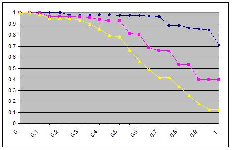
Figure 5. Configuration coverage for 2⁷⁹3¹4¹6¹9¹

Implication for Testing

Even if combinatorial testing is not used, measuring configuration-spanning coverage can be helpful in understanding state space coverage. If we do use combinatorial testing, then configuration-spanning coverage will be 100% for the level of t that was selected, but we may still want to investigate the coverage our test set provides for t+1 or t+2. Calculating this statistic can help in choosing between t-way covering arrays generated by different algorithms. As seen in the examples above, it may be relatively easy to produce tests that provide a high degree of spanning coverage, even if not 100%. In many cases it may be possible to generate additional tests to boost the coverage of a test set.

---

J.R. Maximoff, M.D. Trela, D.R. Kuhn, R. Kacker, "A Method for Analyzing System State-space Coverage within a t-Wise Testing Framework", IEEE International Systems Conference 2010, Apr. 4-11, 2010, San Diego.